One-way ANOVA Part 1

Analysis of variance is often abbreviated ANOVA, and “one-way ANOVA” refers to ANOVA with one independent variable. Whereas a t-test is useful for comparing the means of two levels of an independent variable, one-way ANOVA is useful for comparing the means of two or more levels of an independent variable.

To test whether the means of the three conditions in Festinger and Carlsmith’s (1959) experiment are unequal, select ANOVA → ANOVA from the analysis menu. You should get the following dialog:

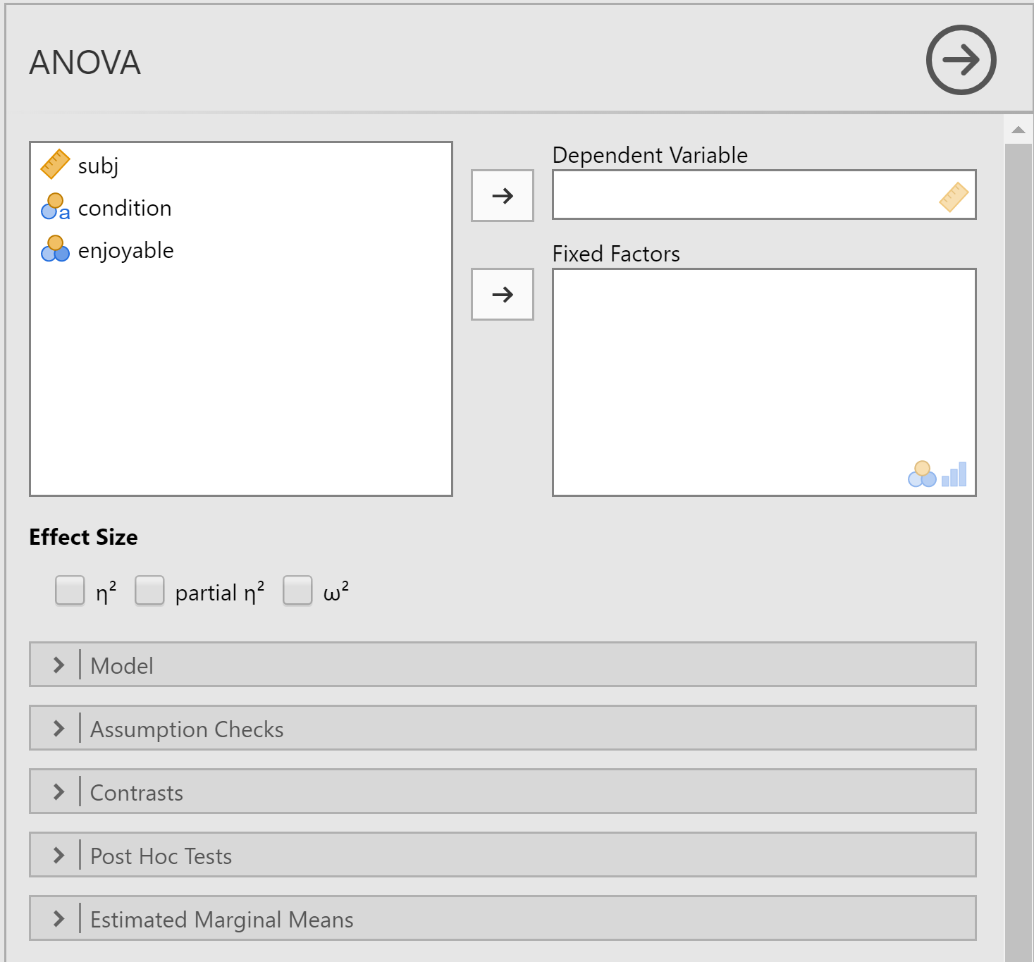
Curse you, JAMOVI trolls!

Hmm...looks like we’ve got something wrong with the dependent variable - enjoyable - but not the independent variable of condition. Jamovi does its best to guess the type of variables, that is, whether the variable is nominal, ordinal or contnuous (interval or ratio). In this case, Jamovi guessed that the dependent variable, as well as the indepndent variable, are nominal. To do an ANOVA, the dependent variable must be continuous, which it is, Jamovi just does not know that. And fortunately, it is an easy change ot make. iables ("Factors") be numbers. We use the same solution as last time: Transform → Automatic Recode:

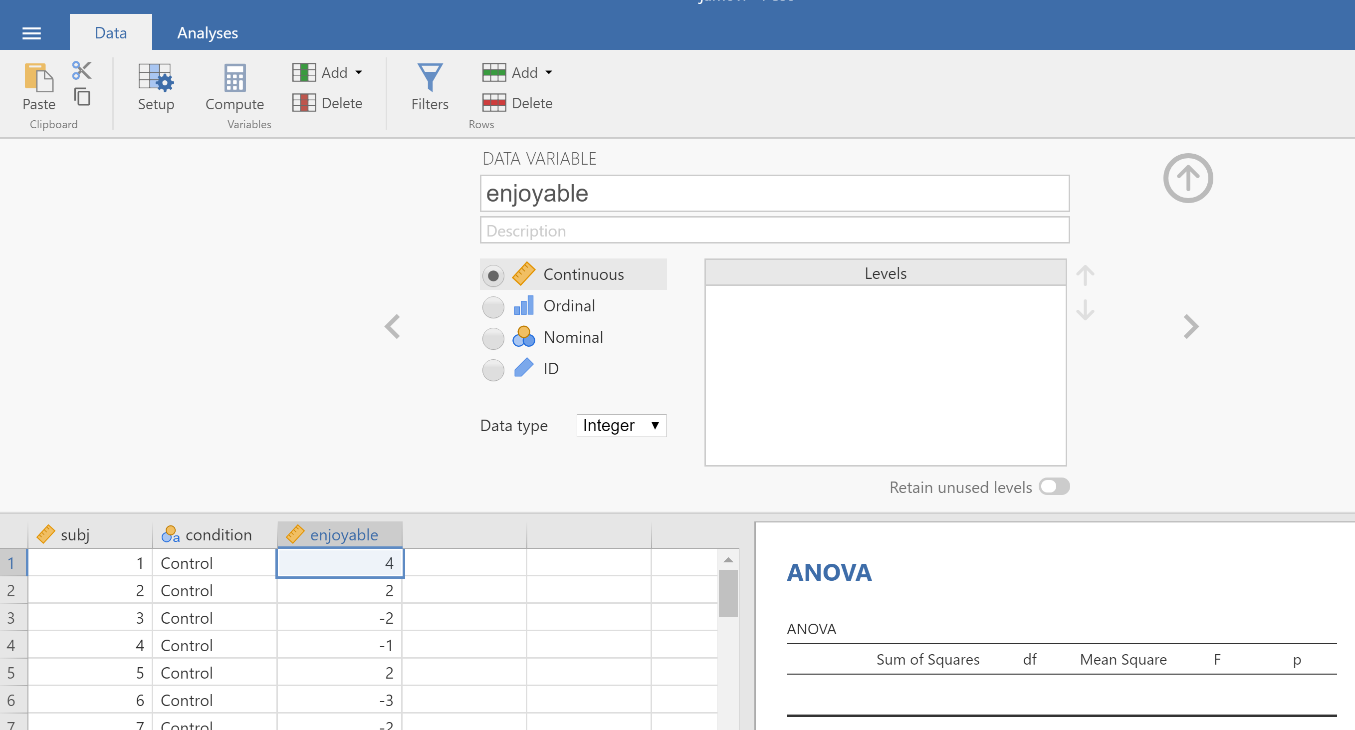
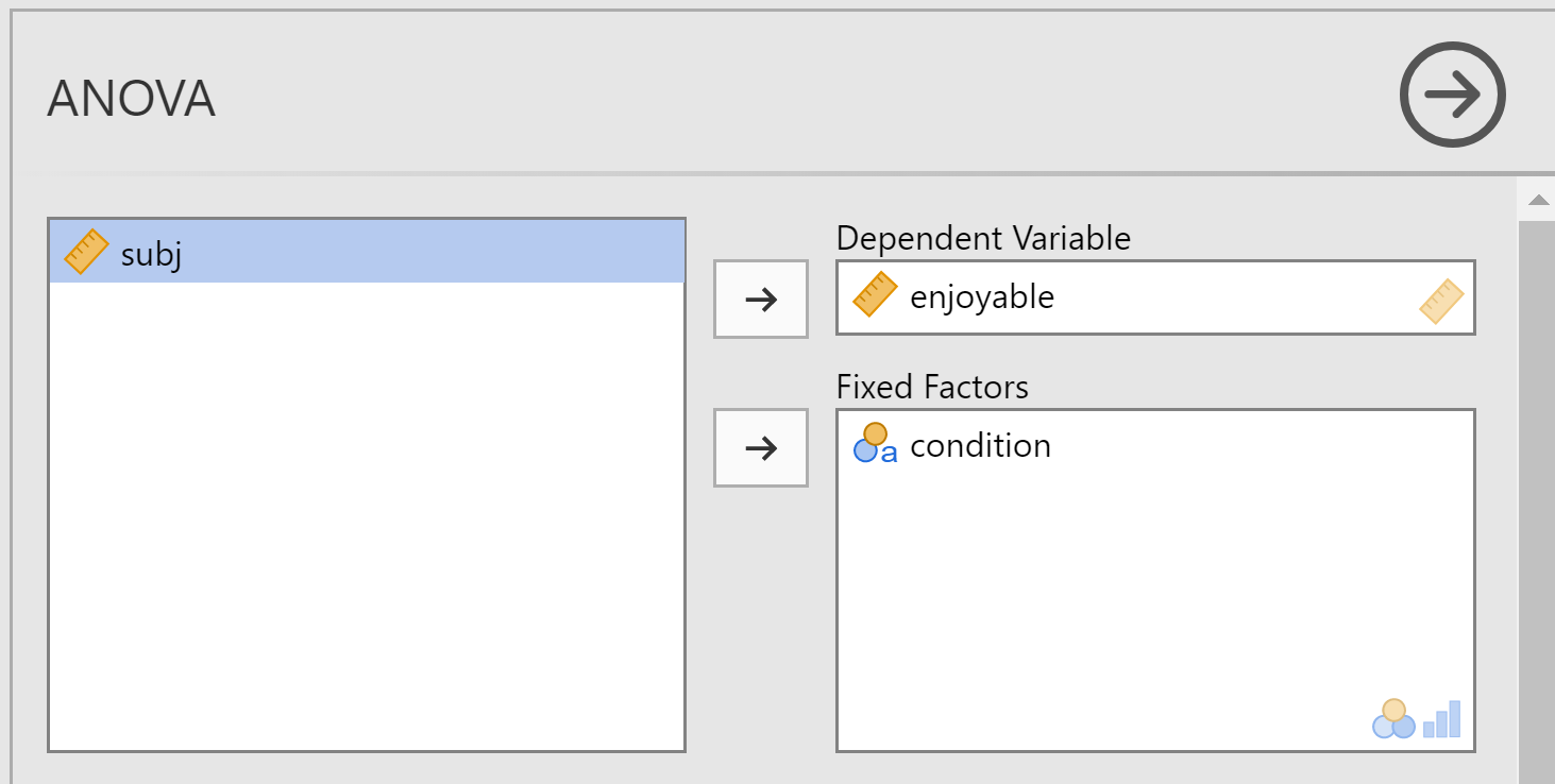
Return to the Anova Dialog by clicking on the ANOVA table in the output window. Move "condition" to "Fixed Factors" and "enjoyable" to "Dependent Variable" like below.

Before you click "OK", first click the "Options" button on the right side of the dialog (under "Contrasts" and "Post Hoc"). Another dialog appears, and you should check the options shown below: "Descriptive" and "Homogeneity of variance test":

Click "Continue" and then "OK". You should get the following output:

ANOVA Output

Testing the null hypothesis that the means are equal

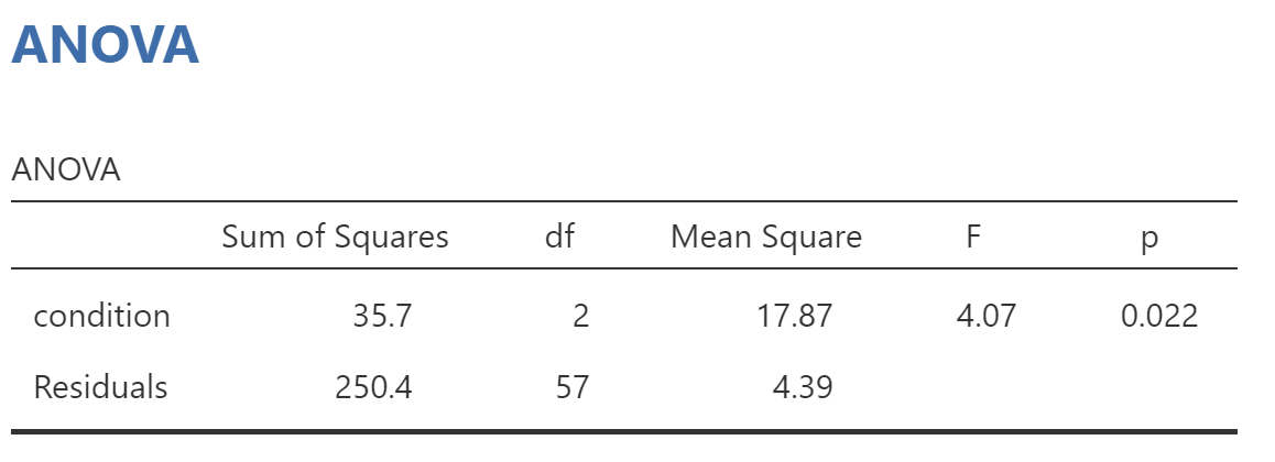
The table above is called an "ANOVA table" and it provides a summary of the actual analysis of variance. Your experimental hypothesis (what you hope to find) is that the means of the three groups are different from one another. Specifically, Festinger and Carlsmith’s experimental hypothesis was that the mean of the One Dollar group will be higher than the mean of the other two groups. The null hypothesis is the "prediction of no effect." In this case, it is that the means of the three groups are equal. The output above estimates the probability that the null hypothesis is true, given the data you obtained. The ANOVA table provides you with the following information:

condition (Between Groups)	Variance is a measure of dispersion, or how spread out the dependent variable is. The word analysis means "a cutting into parts" and this statistical procedure is called "analysis of variance" because it attempts to divide the variance in your dependent variable into two parts: Between Groups and Within Groups. The Between Groups variance is the portion of the variance that can be explained by knowing what group the subjects are in. Since Jamovi knows that this is the condition variable, this line is labeled Condition.
Residuals (Within Groups)	Residuals or Within Groups variance is a measure of how spread out the scores are within each group. In some programs, this will be listed as Error.
df	This stands for "degrees of freedom". For Between-Groups, it is equal to k - 1, where k is the number of levels of the IV. Because Festinger and Carlsmith have 3 levels, df for Between Groups is 2. For Within-Groups, it is equal to N - k, where N is the number of people in your experiment. Because there were 20 people in each condition, there were 60 people total. N = 60. And because there were 3 conditions, the df for Within Groups is N - k = 57.
F	This is the test statistic for ANOVA. Like t, it gets larger as the means of the groups get farther apart (increasing the Between-Groups variance) and it gets smaller as the variability within groups gets larger (increasing the Within-Groups variance). F is the ratio of the Between-Groups variance (listed under "Mean Square") to the Within-Groups variance: 17.867 / 4.394 = 4.066.
Sig.	This is the p-value, expressed as a probability. In this case, p = 0.022. This is the probability of obtaining an F value as large or larger than 4.066, assuming that the null hypothesis is true. The null hypothesis is that the means are equal. Because p is lower than the usual cutoff of p < .05, we would conclude that the means are unequal.

Testing an assumption of ANOVA

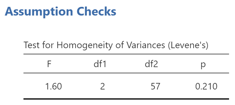
The above table is similar to the Levene’s test that we saw in the output for the t-test. It tests whether the variances in the groups are equal. For the ANOVA to produce an unbiased test, the variances of your groups should be approximately equal. If the value under "Sig." (the p-value) is less than .05, it means that the variances are UNequal, and you should not use the regular old one-way ANOVA. In the table above, p = 0.210, so no problems: you can use the results that follow.

Interpreting the ANOVA output

You tested the null hypothesis that the means are equal and obtained a p-value of .02. Because the p-value is less than .05, you should reject the null hypothesis. You would report this as:

Results from a one-way ANOVA indicated that the means of the three conditions were unequal, F(2,57) = 4.07, p = .022.

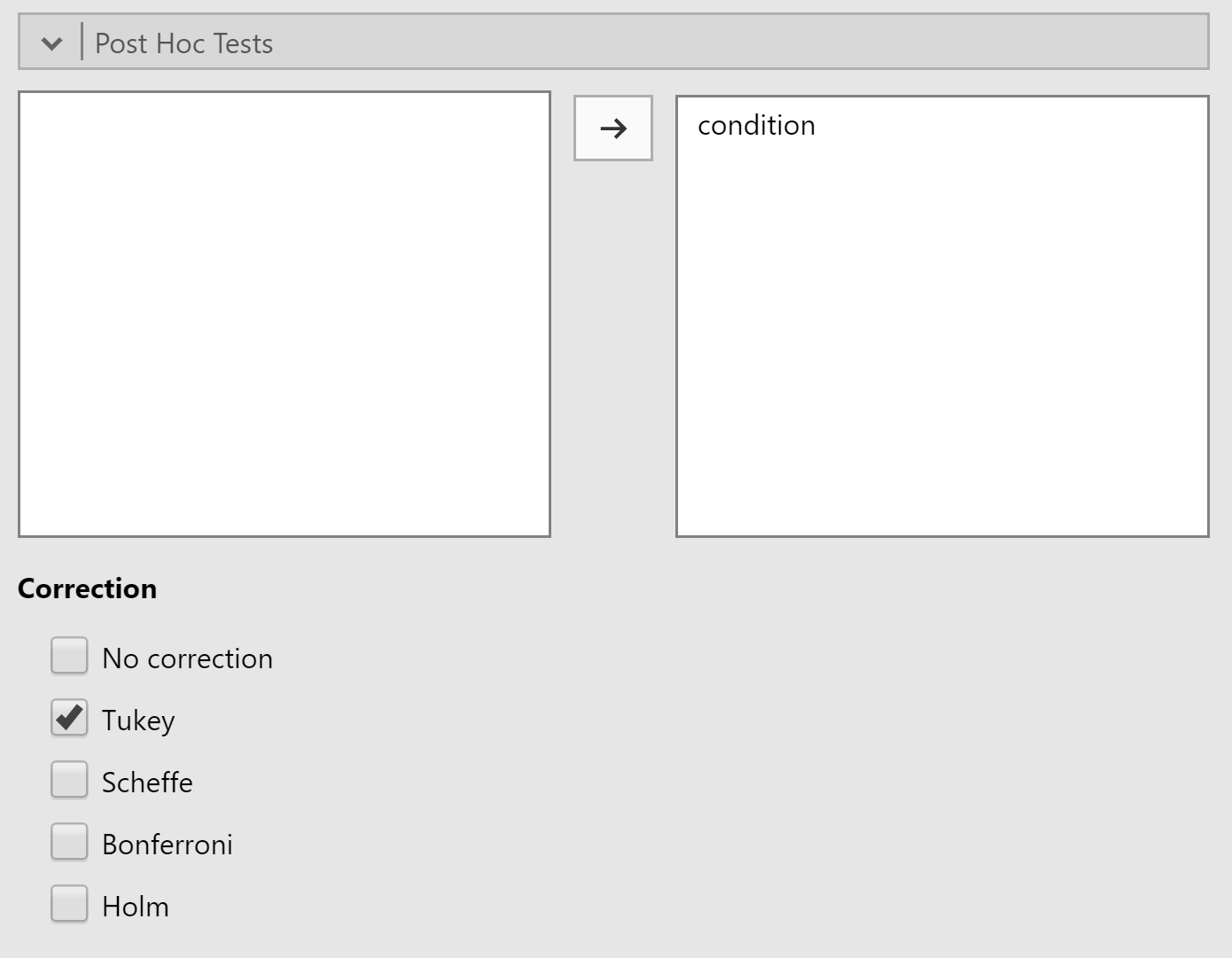
Although you know that the means are unequal, one-way ANOVA does not tell you which means are different from which other means. It would be very nice to know whether the mean in the One Dollar condition was higher than the means of the other two conditions. In ANOVA, testing whether a particular level of the IV is significantly different from another level (or levels) is called post hoc testing. Hey, that sounds familiar! Didn’t we see a dialog heading called "Post Hoc"? Go ahead and open post hoc. You should get this:

 

The multiple comparison problem

If you set your alpha level to .05 (meaning that you decide to call any p-value below .05 "significant"), you will make a Type I error approximately 5% of the time. 5% translates to 1 out of 20 times. That means that if you perform 20 significance tests, each with an alpha level of .05, you can expect one of those 20 tests to yield p < .05 even when the data are random. As the number of tests increases, the probability of making a Type I error (a false positive, saying that there is an effect when there is no effect) increases. The multiple comparison problem is that when you do multiple significance tests, you can expect some of those to be significant just by chance. Fortunately, there is a solution:

Tukey’s HSD

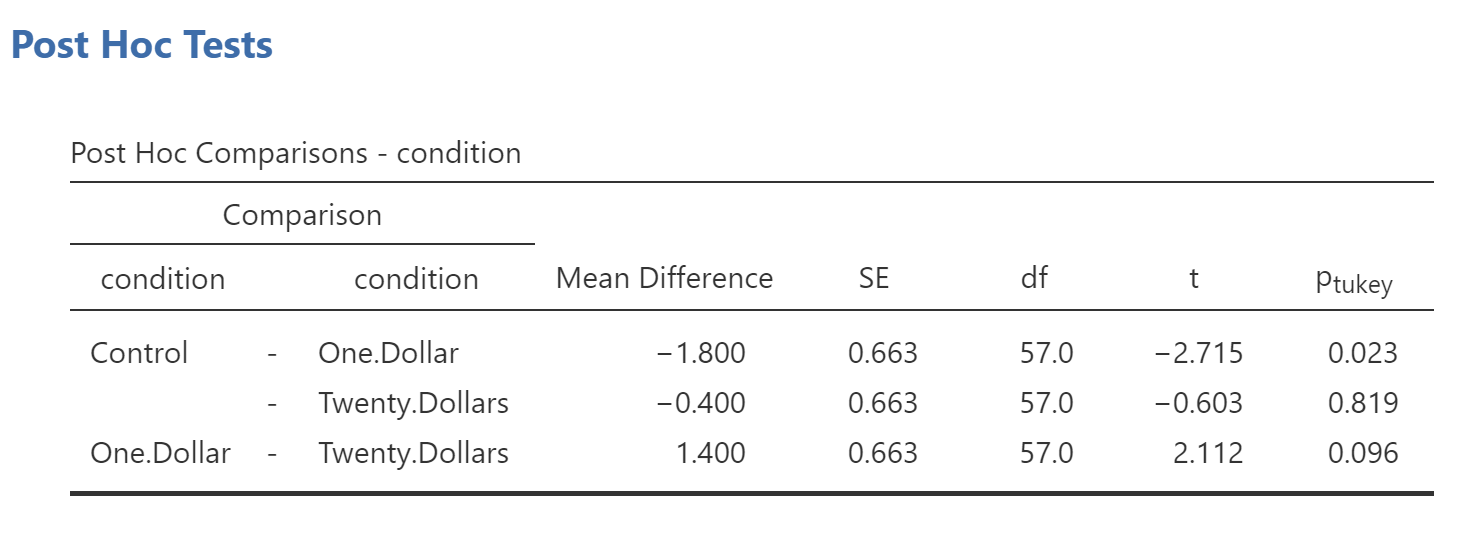
First, note that the first word here is "Tukey", as in John Tukey the statistician, not as in the bird traditionally eaten at Thanksgiving. John Tukey developed a method for comparing all possible pairs of levels of a factor that has come to be known as "Tukey’s Honestly Significant Difference (HSD) test". The results from the ANOVA indicated that the three means were not equal (p < .05), but it didn’t tell you which means were different from which other means. Tukey’s HSD does that: for every possible pair of levels, Tukey’s HSD reports whether those means are significantly different. Tukey’s HSD solves the problem by effectively adjusting the p-value of each comparison so that it corrects for multiple comparisons.

So, in that dialog for Post Hoc Comparisons, check the box next to "Tukey", then make sure "condition" is in the right hand box like shown. Some new output appears:

In the first row of the table above, the Control condition is compared against the One Dollar condition. The mean difference is -1.800 and the p-value, listed as Ptukey, is .023. Because p < .05, you can consider the difference between the Control and One Dollar condition "significant". The other two comparisons (Control vs. Twenty Dollars and One Dollar vs. Twenty Dollars) were not significant because the p-values are above .05.

Writing It Up in APA Style

To report the results of a one-way ANOVA, begin by reporting the significance test results. Then elaborate on those by presenting the pairwise comparison results and, along the way, insert descriptive statistics information to give the reader the means:

The means of the three conditions were unequal according to a one-way ANOVA, F(2, 57) = 4.07, p = .02. Pairwise comparisons of the means using Tukey’s Honestly Significant Difference procedure indicated only one significant comparison: Subjects in the one-dollar condition (M = 1.35) reported that the tasks were significantly (p = .02) more enjoyable than subjects in the control condition (M = -0.45), with a 95% confidence interval of the difference between means from 0.2 to 3.4 points on a -5 to +5 scale. The other comparisons were not significant (ps > .09).

On the next page, we’ll look at a way to present the results of a one-way ANOVA in a table.